AC297R - Google

• Overview
• Motivation
  • What is an Adversarial Example?
• Datasets
• Literature Review
  • Fast Gradient Sign Method
  • Jacobian-Based Saliency Map Approach
  • Projected Gradient Descent
  • Other Attack Methods
  • Adversarial Training
  • Other Defense Methods
  • Adversarial Examples Tutorial
• Application: GTSRB
  • Accuracy vs. Perturbation Trade Off
• Adversarial Training with Data Augmentation
  • Mixup
  • Random Erasure
• Conclusion

Overview

In partnership with Google Brain this project explores the field of adversarial examples, inputs designed to trick neural networks, with the goal of making them more accessible to learn about. Starting with motivation, we explain what adversarial examples are and why they are important. From there we review the datasets we use and the literature of adversarial examples. Finally, we share results we have from testing some experimental adversarial defense methods.

Motivation

As Machine Learning is becoming more ubiquitous, understanding how neural networks are learning is becoming increasingly important. Our project explores the field of adversarial examples, which challenges the common belief that neural networks are learning patterns in the data.

What is an Adversarial Example?

Adversarial examples are inputs that have been crafted specifically to trick a neural network, while still being easily discernible to humans. An example of an adversarial example in the context of image classification can be seen below: 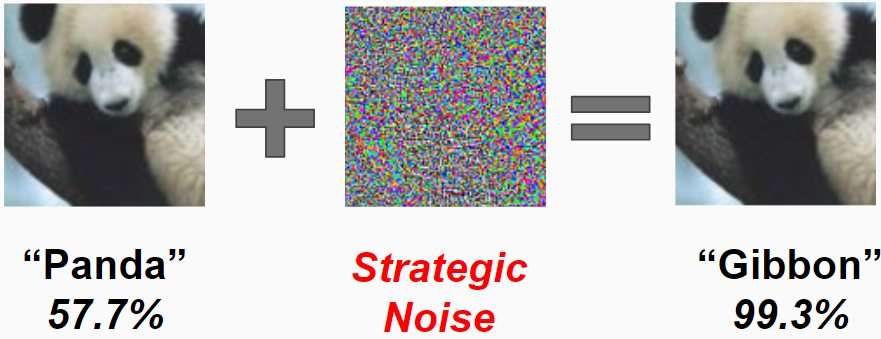While both the left and right images look like a panda, the right image is improperly classified as a gibbon. This misclassifciation is caused by the addition of strategic noise. The existence of such examples calls into question how and what neural networks of learning.

Datasets

For this project we worked on the MNIST, CIFAR-10, and GTSRB datasets. We decided to use MNIST and CIFAR-10 because our project was heavily research focused, and most of the literature worked on image classification on these two classic datasets. This decision made it easy for us to compare model performance to the literature and iterate quickly on experimental model setups. We used the GTSRB dataset as a starting point for an application to driverless cars because the dataset is images of traffic signs.

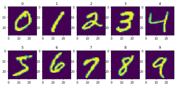
The MNIST dataset is a classic image classification dataset that features 28x28 greyscale images of handwritten digits. There are 10 classes (digits from 0-9), and the dataset contains 60,000 training examples and 10,000 test examples. Below are some images from the MNIST dataset:

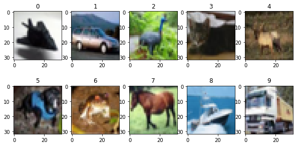
CIFAR-10 is another image classification dataset that contains 32x32 color images of 10 classes. Classes consist of various objects and animals such as airplanes, deer, and trucks. There are 60,000 training example sand 10,000 test examples. Below are some images from the CIFAR-10 dataset:

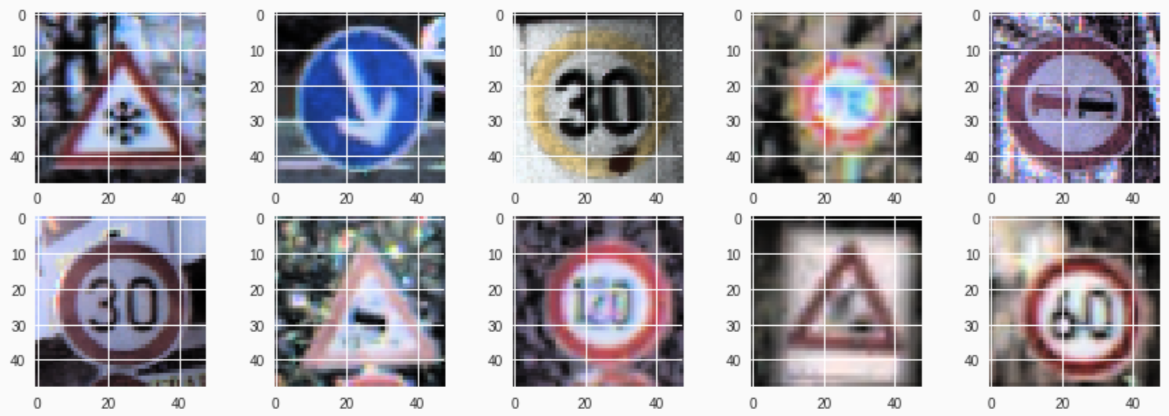
The GTSRB (The German Traffic Sign Recognition Benchmark) dataset consists of images ranging in size from 15x15 to 250x250 of German traffic signs. There are 43 distinct classes of signs and over 50,000 total images. Below are images from the GTSRB dataset:

Literature Review

Adversarial examples are relatively new to the machine learning community, yet they have already accumulated a rich history in literature.

Research on adversarial examples can be broadly classified into two main avenues. Many of the earliest results focused on attack methods for systematically generating images that fool advanced machine learning models to into misclassifying the input. Recently, there has been much interest in analyzing the other side of the coin - i.e. defense methods for protecting models against adversarial attacks.

In this section, we give a quick overview of the attack and defense literature, placing special emphasis on the results that are most pertinent to our own research project.

Attack: Fast Gradient Sign Method (FGSM)

The concept of an adversarial example was invented by Szegedy et al. in 2013 ¹ and formalized by Goodfellow et al. in 2014 ². In the same paper, Goodfellow et al. introduced Fast Gradient Sign Method (FGSM), which is a simple and intuitive way to generate adversarial examples.

Let’s say we have an input image $\vx \in \X$ that we wish to transform into an adversarial example $\vx' \in \X$, where $\mathcal{X}$ is the space of all possible images. Let the model we wish to attack have pre-trained parameters $\vect{w} \in \R$ using some loss function $\ell : \mathcal{X} \times \R \to \R^+$. Then, given a step size parameter $\epsilon$, FGSM generates $\vx'$ with the following gradient update:

where $\sgn$ is the vectorized sign function. The intuition for FGSM comes from the idea that adversaries would want to slightly perturb the original image $\vx$ in the direction of the loss function’s gradient, so that $\vx'$ corresponds to a higher loss than $\vx$. Here we use the sign of the gradient instead of the actual gradient so as to ensure that each pixel of $\vx$ is perturbed by at most $\epsilon$ — a change that should be unrecognizable to the human eye.

Note that FGSM is an untargeted attack, because the adversary has no control over which specific class the model will classify $\vx'$, since $\vx'$ was created with the sole purpose of increasing the loss function $\ell$ as much as possible.

Attack: Jacobian-Based Saliency Map Approach (JSMA)

In 2016, Papernot et al. published an effective adversarial method for targeted attacks called the Jacobian-Based Saliency Map Approach (JSMA)³. Let the original image of $N$ pixels be $\vx$ with true class $k \in \{1, \ldots, K\}$ where $K$ is the total number of possible classes. Let $\vy$ be a $K$-dimensional one-hot encoding of $k$. In a neural network with parameters $\vect{w}$, the loss function $\ell$ is commonly defined as the cross-entropy between the data’s distribution and the model’s distribution,

where $\cdot$ denotes the dot product and $\vect{f}(\vx, \vect{w})$ is the $K$-dimensional output of the final layer of the neural network. Note that $\vect{f}$ is also a vector of probabilities in which the $j$th entry denotes the probability that the neural network assigns to class $j$.

JSMA is centered around computing the Jacobian matrix $J$, an $N$-by-$K$ matrix where entry $(i, j)$ is defined as

Intuitively, we can think of $J_{i, j}$ as how much we would increase the probability of the neural network classifying the image as class $j$ if we were to slightly perturb pixel $i$. Now, suppose an adversary is interested in constructing an adversarial example $\vx'$ that the neural network will foolishly classify as some target class $k' \neq k$. Then, the adversary can simply do the following:

1. Compute the Jacobian matrix $J$ for the current image $\vx$.
2. Use $J$ to identify a couple of pixels that we can perturb to decrease the probability of class $k$ and increase the probability of class $k'$.
3. Make these perturbations to create an adversarial image $\vx'$.
4. Update $\vx \leftarrow \vx'$. Repeat steps 1-3 until the network misclassifies $\vx$ as target class $k'$.

Note that unlike FGSM, JSMA applies strategic perturbations to specific pixels instead of uniformly changing the entire image. Though this method is quite effective at targeted misclassification, it is computationally expensive because the Jacobian matrix must be recomputed at each iteration of the attack.

Attack: Projected Gradient Descent (PGD)

Projected Gradient Descent (PGD) is an iterative application of FGSM on the loss function $\ell$. It was created by Madry et al. in 2017 ⁴. Let $\vx$ be the original image with $N$ pixels. The parameters of PGD are the maximum distortion parameter $\epsilon$ , the step size parameter $\alpha$, and the number of iterations $T$. At each iteration $t \in \{1, \ldots, T\}$ of PGD, the attack algorithm will produce a newly perturbed image $\vx^t$. The final output will be the created adversarial example $\vx' = \vx^T$.

PGD differs from FGSM in two main ways. First, the authors found that randomly initializing the starting point of the gradient ascent leads to more robust adversarial results. Thus, PGD begins by choosing a starting point uniformly at random from within an $N$-dimensional hypercube centered at $\vx$ with side length $\epsilon$. Second, PGD performs not one, but $T$ steps of the basic FGSM algorithm with step size $\alpha$. At any given point, we may need to clip the perturbations to ensure that the cumulative distortion from the original example $\vx$ does not exceed $\epsilon$ for all pixels. The full PGD algorithm is given below.

1. Let $\vx^0 = \vx + \epsilon \cdot \vect{\delta}$ where $\vect{\delta} \sim \text{Uniform}(\vect{0}, \vect{1})$.
2. For each iteration $t \gets 1, \ldots, T$
   1. Do an FGSM step and compute $\begin{align*} \vx^t = \vx^{t-1} + \alpha \cdot \sgn \left(\frac{\partial \ell}{\partial \vx^{t-1}}\right) \end{align*}$.
   2. For each pixel $p \gets 1, \ldots, N$
      1. If $x^t_p - x_p > \epsilon$, then clip the cumulative perturbation by setting $x^t_p = x_p + \epsilon$.
      2. If $x^t_p - x_p < -\epsilon$, then clip the cumulative perturbation by setting $x^t_p = x_p - \epsilon$.
3. Return adversarial example $\vx' = \vx^T$.

The intuitive advantage of PGD over FGSM is that the former takes small steps to iteratively approximate the gradient instead of taking one large step like the latter. Thus, PGD is able to increase the loss function more efficiently.

Attack: Other Methods

Our research focused on the aforementioned attack methods, but there are many more in literature. These include the Iterative Least-Likely Class Method (ILLC), Carlini and Wagner’s Attack (C&W), Zeroth Order Optimization (ZOO), and more. A comprehensive list can be found in Yuan et al.’s 2017 literary review ⁵.

All of the methods mentioned thus far are known as “white box” attacks, because they require the adversary to have access to the model’s parameters in order to generate adversarial examples. However, in 2016, Papernot et al. introduced a generic strategy for transferring these “white box” methods into “black box” ones in which such parameters are unknown ⁶. An adversary can use this method as follows,

1. Observe input images $\{\vx^1, \vx^2, \vx^3, \ldots\}$ that are fed into a model and the corresponding classifications $\{\vy^1, \vy^2, \vy^3, \ldots\}$ that come out.
2. Use this set of pairs $\{(\vx^1, \vy^1), (\vx^2, \vy^2), (\vx^3, \vy^3), \ldots\}$ as the training set for a neural network that will mimic the behavior of the original model (which is treated as a “black box”).
3. Generate an adversarial example $\vx'$ for the mimicking neural network using an aforementioned “white box” attack.
4. Feed the adversarial example $\vx'$ to the original model. It should force the original model to misclassify, assuming that the mimicking neural network is accurate in matching the original model’s behavior.

Defense: Adversarial Training

Goodfellow et al. established the first known method of preparing models to defend against adversarial examples in their seminal 2014 paper ². Adversarial Training is the simple idea of building adversarial examples into the training set. More specifically, during the training procedure of a neural network, let there be an image $\vx$ with true class $\vy$. The network has parameters $\vect{w}$ and a loss function $\ell$ that we can use to generate an adversarial examples $\vx'$ via one of the attack methods introduced earlier. Then, we can add $(\vx', \vy)$ to the original training set and our model will have seen adversarial examples during training, thereby making it more robust to future attacks.

Defense: Other Methods

Adversarial Training has proven to be quite an effective measure for defending against adversarial examples. In fact, it is arguably the only robust defense method that has been invented. Many other proposals, such as Adversarial Detecting, Ensembling Weak Defenses, and Gradient Hiding, have been shown to be easily defeated in practice ⁵.

Therefore, part of our research project involved investigating new data augmentation methods that could be used in concert with adversarial training to defend against adversarial examples. Specifically, we explore mixup and random erasure as data augmentation techniques.

Adversarial Examples Tutorial

We have created a Jupyter Notebook-based tutorial on how to create and defend against adversarial examples. The tutorial uses the CleverHans Library in concert with Keras to teach attack/defense methods on simple datasets such as MNIST and CIFAR-10. You can access this tutorial here.

Application: GTSRB

We used the GTSRB dataset to simulate how adversarial attacks and defenses would work in the setting of driverless cars. In addition to having the properties mentioned in the above section, the GTSRB dataset also has some adversarial literature that we benchmark against. Aung et al demonstrate many of the aforementioned attack and defense methods on GTSRB and experiment with methods for making neural networks more robust ⁷.

Accuracy vs. Perturbation Trade Off

In the paper by Aung et al, the step parameter, $\epsilon$, for FGSM is analyzed to see how it affects accuracy ⁷. We furthered this analysis by testing if we could use the Gini coefficient to determine an optimal $\epsilon$ that would significantly reduce the classifier’s accuracy while preserving the original image. We use Gini as a measure of the impurity because higher Gini values indicate a very uncertain classifier and that the image is closer to random noise.

Below are four adversarial examples of the same traffic sign with different $\epsilon$ parameters:

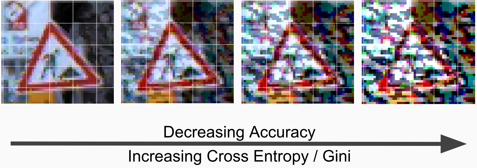
The images on the left side have smaller $\epsilon$’s and resemble the original image quite well. As $\epsilon$ increases, however, the image becomes more perturbed and eventually more like random noise than an actual sign. To see how $\epsilon$ affects accuracy and Gini we swept over a range of $\epsilon$’s and found the accuracy and Gini of the test set for each $\epsilon$.

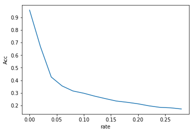
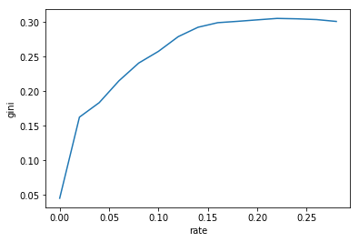
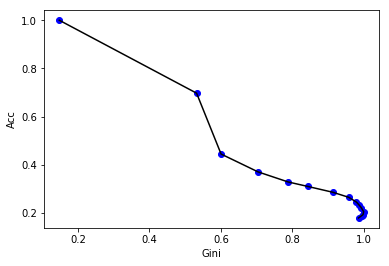
These are plots that show how accuracy and Gini change as $\epsilon$ increases. As expected a larger $\epsilon$ reduces accuracy and also increases the Gini coefficient. In order to pick an optimal value we plotted Accuracy vs Gini and tried to use the elbow method to find an epsilon that balanced accuracy and input impurity.

Adversarial Training with Data Augmentation

A major component of this research project involved investigating ways to train models for defense against adversarial examples. Upon consulting with our Google partner, we identified combining adversarial training with data augmentation as a promising research direction. Data augmentation is a process in which we somehow alter the training data before using it to train the model. The specific data augmentation methods that we examined are mixup and random erasure. Work on mixup seems promising, yet we mostly obtained negative results for random erasure.

Mixup

In 2017, mixup was introduced by Zhang et al. as a method to construct virtual training examples by interpolating between two different points in the training set ⁸. First, choose two images $\vx^i$ and $\vx^j$ that belong to two different classes $\vy^i$ and $\vy^j$. Note that $\vy^i$ and $\vy^j$ are one hot-encoded. Then, mixup generates a new image $\tilde{\vx}$ with a new class $\tilde{\vy}$ that is defined as follows:

for some value $\lambda \in [0, 1]$. The original authors chose to draw $\lambda$ from a $\text{Beta}(\alpha, \alpha)$ distribution, where $\alpha$ is a predetermined hyper-parameter. This new image $\tilde{\vx}$ is a linear interpolation between the two original images and has a corresponding class $\tilde{\vy}$ that is the same linear interpolation between the two original classes. We add this newly constructed pair $(\tilde{\vx},\tilde{\vy})$ to our training set.

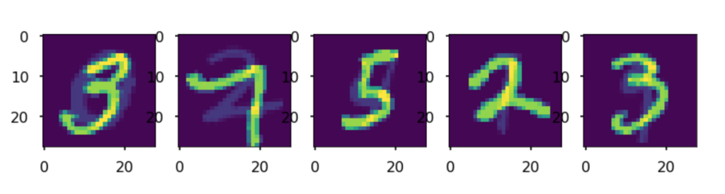
Here are some examples of mixup on MNIST images.

The intuition behind mixup is that it can help the model “smooth out” decision boundaries between two different classes by letting it train on points between them. If points from class A and class B are well-separated, then the decision boundary assigned by the model could fluctuate between being very close to points in class A and being very close to points in class B. However, with mixup, we can ensure that the decision boundary will be halfway between the class A points and the class B points. Thus, an adversary will be less likely to take advantage of a sharp decision boundary in using gradient ascent-based methods to create adversarial examples. In fact, Zhang et. al present some results showing that training models with mixup can improve robustness to adversarial examples on the ImageNet dataset ⁸.

Our contribution mainly involved combining mixup with adversarial training.

Here are some results from our experiments. We tested how five models that were trained differently (i.e. Normal, Mixup, Adversarial Training, Mixup Adversarial Training, Adversarial Mixup Training) reacted to adversarial attacks on the MNIST dataset. The y-axis denotes “Adversarial Accuracy” (i.e. the accuracy that each model achieved on classifying adversarial examples that were generated using FGSM). It is a function of the x-axis, which varies the FGSM parameter $\epsilon$ that was used in the attacks.

The different models varied in the ways in which their training sets were preprocessed. The “Normal” model was trained in a standard manner with no adversarial training and no data augmentation. The “Mixup” model was trained using mixup and the “Adversarial Training” model was trained using FGSM-based adversarial training. The “Mixup Adversarial Training” model first mixed up images and then applied adversarial training to these images. The “Adversarial Mixup Training” model did the opposite – first generating adversarial images and then mixing those adversarial images up. All models used the same basic architecture – a simple, feedforward neural network with a couple of hidden layers.

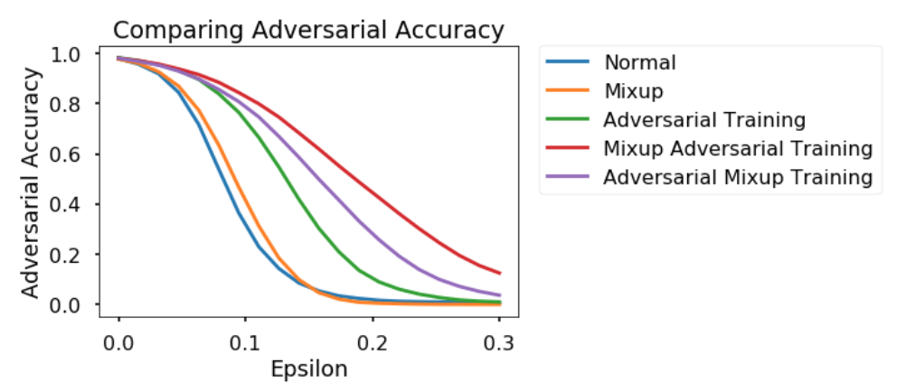
The results show that the “Mixup Adversarial Training” model performed the best in defending against adversarial attacks. Both this model, and the “Adversarial Mixup” model, proved to be more effective for this dataset than either the simple “Adversarial Training” model or the simple “Mixup” model. This suggests that combining adversarial training with mixup may hold some promise in defending neural networks.

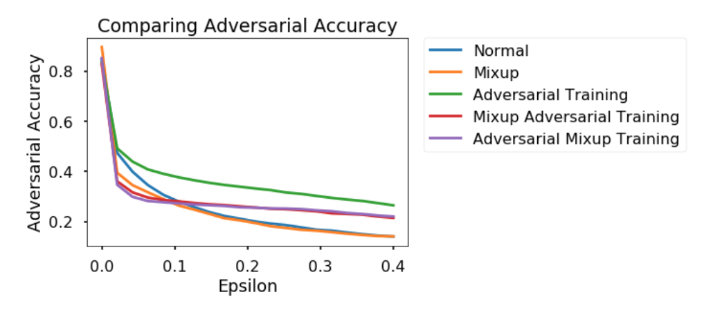
Here is the same experiment done on CIFAR-10. These are the results. They show some positive relationships, but are less supportive of the idea that mixup provides some additional support to adversarial training.

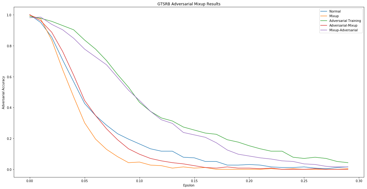
We repeated the same experiment on the GTSRB dataset using PGD instead of FGSM.

Random Erasure

Random erasure is another data augmentation method that was originally designed by Zhong et al. in 2017 as a way to help convolutional neural networks fight overfitting ⁹. We explore random erasure in concert with adversarial training as an adversarial defense strategy.

The idea behind random erasure very simple: given an image $\vx$, cut out a randomly chosen rectangular region and replace it with randomly generated pixels to create an augmented image $\tilde{\vx}$. The class of the augmented image $\tilde{\vy}$ is the same as the class of the original image $\vy$. The pair $(\tilde{\vx},\tilde{\vy})$ is added to our training set.

Here is an example of a CIFAR-10 image with random erasure applied to it.

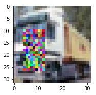
By blocking out parts of an image, random erasure is designed to prevent models from attending to random patches in the background of an image, thereby helping them “learn” better.

We investigate if random erasure can be used to improve the robustness of models with respect to adversarial examples. We consider the efficacy of random erasure both alone and with adversarial training.

Here are the results using FGSM on a CIFAR-10 dataset.

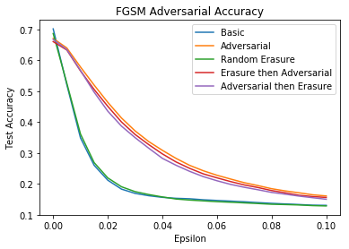
From this graph, we see that random erasure provides no improvement over the basic model and also no additional improvement over a model with adversarial training. Therefore, this method of data augmentation looks less promising than mixup.

Conclusion

In this project, we explored the growing field of adversarial examples, looking at both attack and defense techniques. Adversarial examples are certainly an important aspect of machine learning that must be examined further, as they illustrate how powerful neural networks that are ubiquitous in daily life can be easily fooled. From our defense research, we conclude that mixup shows some promise of being a useful defense tactic, especially when combined with adversarial training. In the future, we would definitely like to explore how other methods can be used to form effective defenses. On the attack side, it would be interesting to look into adversarial examples on discrete input spaces (such as language) and how to construct them when computing the gradient is not possible.